Automatic Feature Extraction: An Introduction to Deep 1D Convolution Networks

Context

As a part of my work in the Anomaly Detection Project, I looked at ways of benchmarking our algorithms performance with standard anomaly detection algorithms in the sensor array literature. One particular model that struck me as interesting was the 1D convolution network (for literature references, see 1 and 2). I was already familiar with the widespread use of 2D convolutions for object detection in computer vision, but had never thought about how these convolutions might be used in time series analysis.

Time series data is often some of the more difficult data to analyse from a statistical point of view. There is often a large quantity of data points; data compression is almost always necessary for computational power, and any model we use must take into account the autocorrelation (i.e. correlation in time) of the data. Feature extraction is a common first step in analysing time series; this involves compressing a given time series into a number of features which (hopefully) characterise the data without losing any information. Future analyses would focus on working with this set of features with typical statistical techniques such as clustering (k-means), machine learning algorithms (random forests, support vector machines, neural networks), regression and so on. However, this process is often fraught with danger. Features that return state-of-the-art results in one area often perform very poorly in another. For example, in our anomaly detection project, I tried to use state-of-the-art features for electroencephalogram (EEG) data classification (see 3) with a tuned SVM; in our (heavily noise-affected) domain, such features barely outperformed random guessing.

This is where 1D convolution networks come in. 1D convolution networks remove the need for domain expertise and manpower spent on manual feature extraction. Feeding in raw time series data, 1D convolution networks process the data through multiple layers of “moving average windows” (filters) before combining the predictions in a final dense layer. By optimising the weights in each filter using standard backpropagation algorithms (ADAM), we can train a network to categorise time series data just as we do for images.

Below, we discuss the theory in more depth, present some of my work in applying 1D convolution learning to supervised classification problems and evaluate their performance in the context of algorithm performance and applicability in anomaly detection.

Theory

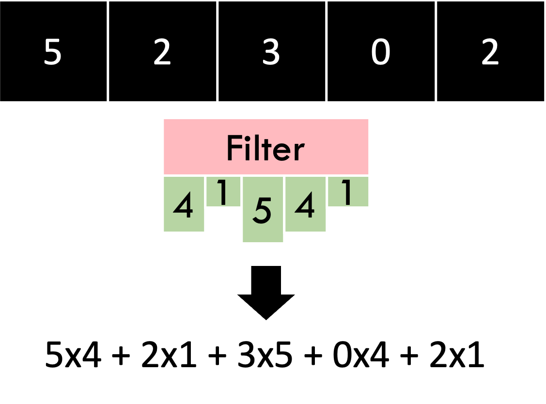The basic operation we need to be familiar with is the “convolution” operation. Given a 1D block of data, we can convolve it with a filter (or window) of weights, which just means to take the dot product of the two vectors together to obtain a single number. That’s all there is to it!

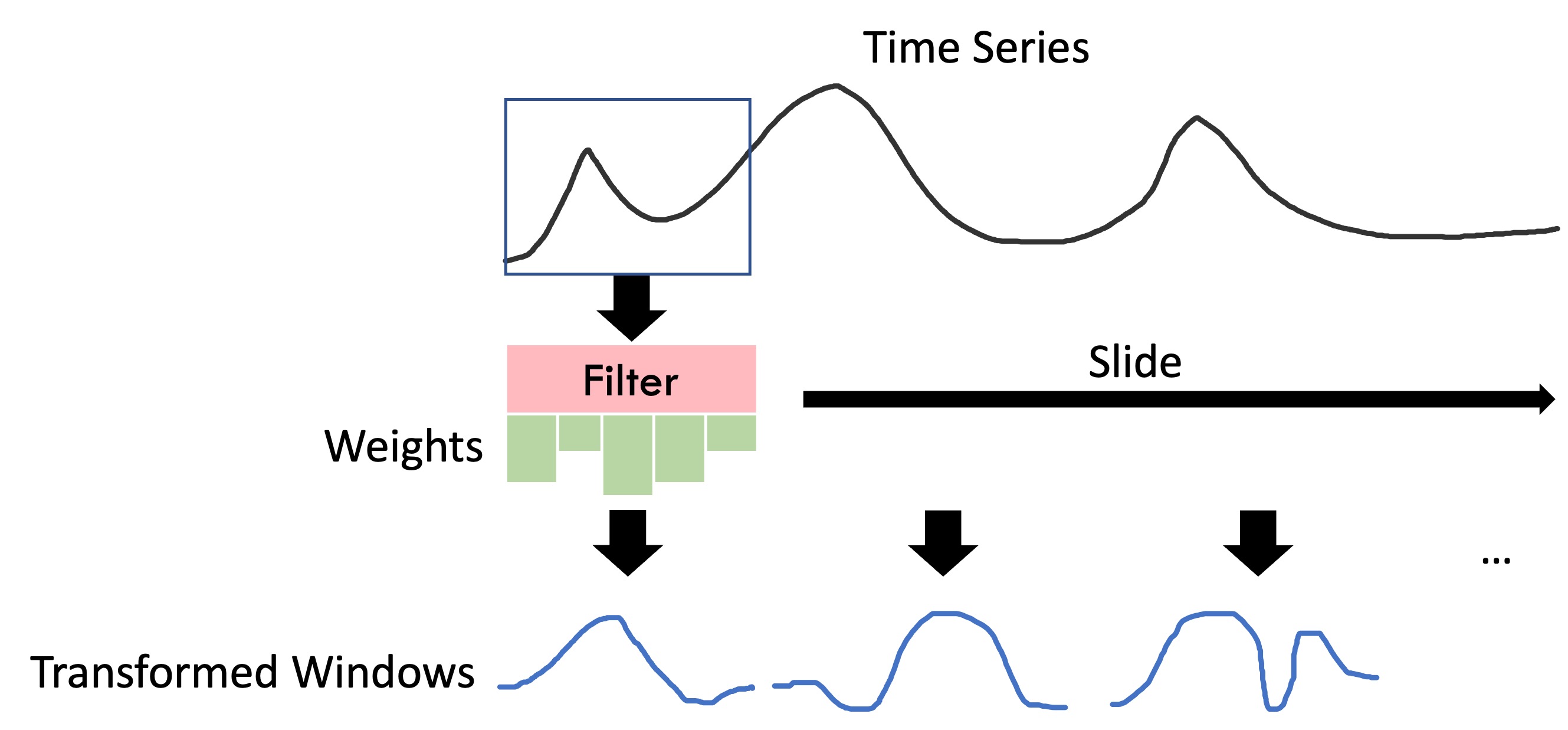
We take a filter and slide it through the time series, taking the convolution at each step to produce a single number. The output of this filter will just be these numbers concatenated into a single vector, which produces another time series. Since this operation will reduce the size of the input, we can pad the original time series by adding in empty blocks (zeros) on the side so that the input and output time series are the same size.

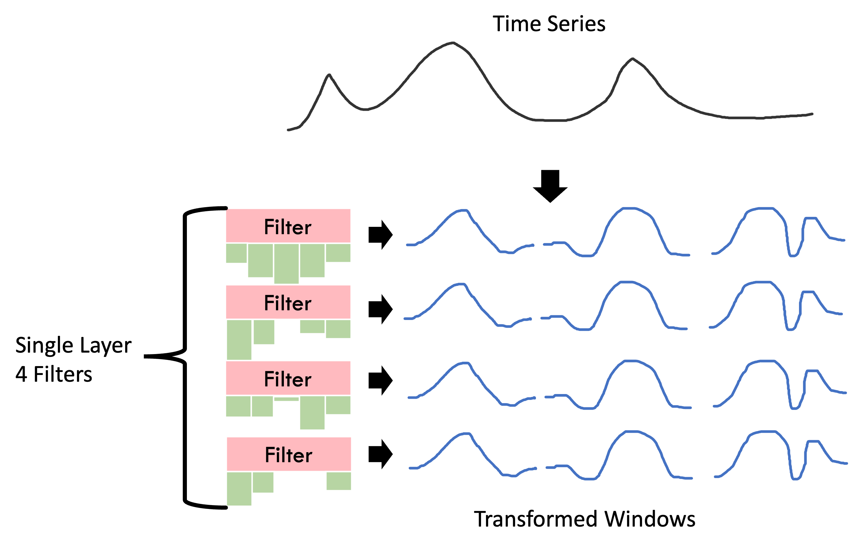
Now that we have convolution filters, we can build up a single convolution layer by stacking together multiple filters. Each filter has its own fixed set of weights independent of the weights of the other filters in its layer. The weights of each filter are optimised to capture some unique feature of the signal, analogous to how 2D convolution filters capture features such as edges in images. Each filter operates independently to the other filters and layers until the final dense layer.

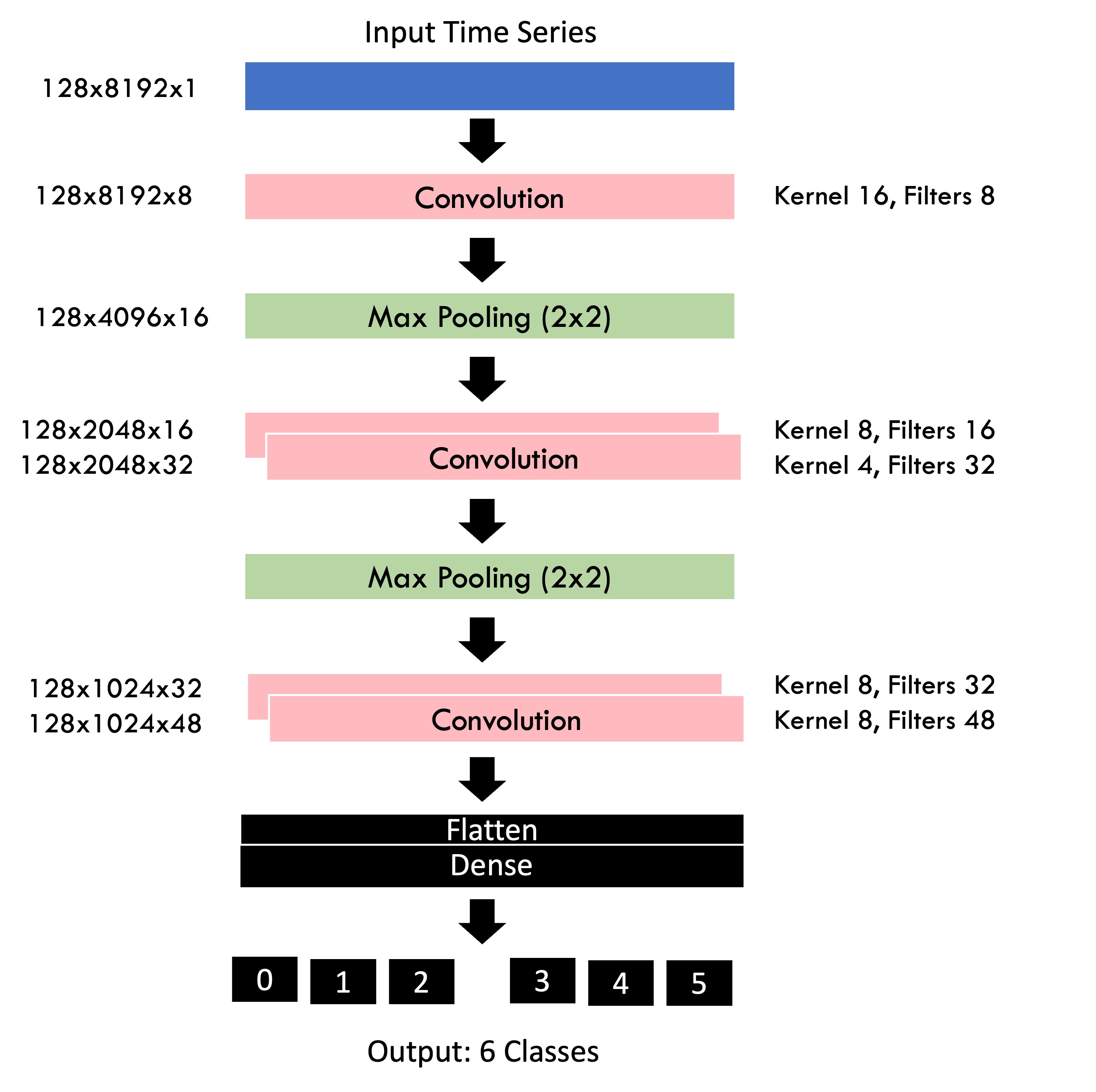
We use 1D max pooling layers in-between convolution layers to reduce computation complexity, and a final dense layer to combine all the features together. After the forward pass, we can evaluate the networks fitness using a loss function (usually mean square error or 0-1 loss), and use an optimisation algorithm to shift all the weights in each convolution layer in the direction that minimises this loss function. By stacking all of these layers together, we can create a deep end-to-end anomaly predictor which takes in raw data and outputs the most likely class directly. The image above is the network that was implemented in my project.

Data Description

I provide some implementations of 1D convolution networks in Tensorflow on a number of data sets. The first is the Sandia Laboratories Experimental Structure Data (the bookshelf data set), and the second is the Airbus Helicopter Anomalies Data set (the helicopter data set). In both cases, the goal is to categorise each time series into a class based on the amount of damage sustained by the structure. In the bookshelf data set, we are given the exact level of damage applied to the structure before the structure was shaken by a motor. In the helicopter data set, we are not given much information at all, aside from the true class of a given data point.

Bookshelf Data Set

The data description can be found here.

Helicopter Data Set

See here for the source of the data.

Implementation

Please see my GitHub repository here for the notebooks and code.