Recurrence and Transience in Simple Random Walks (The Adventures of Drunk Ants, Men and Bees)
Recently (March/April 2022), my stochastic processes class started discussing Markov processes and the concept of recurrence and transience. Some of the most well-known results in this area concern simple random walks on \(\mathbb{Z}^d\) and their transience and recurrence properties depending on the dimensions \(d\) (I have seen these referred to as Pòlya’s Random Walk Theorems online). The results of these theorems admit some very intriguing, easily accessible analogies: “drunk ants and men will surely find their way home, but a drunk bird may get lost forever”. In honour of how catchy this analogy is, I decided to write up a post with some definitions, proofs and silly pictures. Let’s do it!
We begin by defining a simple random walk. We will only concern ourselves with walks in time \(T = \{0,1,2, \dots\}\) and on the state space \(\mathbb{Z}^d\) for \(d \geq 1\).
Definition 1. A simple random walk is a discrete stochastic process \((X_n)_{n \in T}\) on the state space \(\mathbb{Z}^d\) such that at every time step, exactly \(1\) of the coordinates changes by \(+1\) or \(-1\), with all such transitions occurring with equal probability.
For example, the simple random walk with \(d = 1\) starting at \(0\) is a sequence that increases by \(1\) or decreases by \(1\) with probability \(1/2\) each. The simple random walk on \(\mathbb{Z}^2\) starting at \((0,0)\) has four possible positions to move to in the first timestep (these are \((0,1), (1,0), (-1,0), (0,-1)\)) and hence each transition occurs with probability \(1/4\), and so on.
Definition 2. A simple random walk on \(\mathbb{Z}^d\) is said to be recurrent if, for any state \(x \in \mathbb{Z}^d\), the probability that the walk will return to \(x\) in finite time is equal to \(1\). Otherwise, it is said to be transient.
Recurrent walks will always, at some point, find their way back to where they started. Conversely, transient walks have a positive probability of disappearing infinitely far away, never to return. We can write \(N_x\) to denote the random variable
\[N_x = \sum_{n=1}^\infty 1_{X_n}(x),\]which represents the number of times the random walk returns to \(x\). In this notation, the recurrence property can be written as the fact that there exists some state \(x\) such that
\[P(N_x \geq 1) = 1\]The expected number of returns is given by the expectation
\[\mathbb{E}N_x = \sum_{n=1}^\infty P(X_n = x)\]Of course, we invoke Fubini’s theorem to justify the interchange of the infinite sum and expectation (I wouldn’t catch you doing this without justification, would I?). It can be shown that the expected number of returns \(\mathbb{E}N_x\) characterises recurrence in random walks (indeed, for Markov chains in general), with the following result:
Proposition 1 For simple random walks, we have the equivalence
\[\mathbb{E}N_x = \infty \text{ for any } x \in \mathbb{Z}^d \iff (X_n)_{n \in T} \text{ is recurrent.}\]Proof: Firstly, by the tail sum formula we can write the expected number of returns to \(x\) as the sum over the probabilities
\[\mathbb{E}N_x = \sum_{n \geq 1} P(N_x \geq n)\]where \(P(N_x \geq n)\) denotes the probability that the number of returns to \(x\) is greater than \(n\).
Write \(T_{x,n}\) as the random variable denoting the duration of the \(n\)th “excursion” from \(x\) (that is, after returning to \(x\) \(n-1\) times, how long does it take the walk to return to \(x\) next?). Then each \(T_{x,n}\) is independent and follows the same distribution for all \(n\). The probability that the number of returns to \(x\) being greater than \(n\) is given by
\[P(N_x \geq n \mid X_0 = 0) \\ = P(T_{x,1} < \infty, P_{x,2}< \infty , \dots, T_{x,n} < \infty \mid X_0 = 0) \\ = P(T_{x,1} < \infty \mid X_0 = x)^n,\]and so by the tail sum formula, we have
\[\mathbb{E}(N_x \mid X_0 = x) = \sum_{q \geq 1} P(T_{x,1} < \infty \mid X_0=x)^q.\]Of course, if \((X_n)_{n \in T}\) is recurrent, then \(P(T_{x,1} < \infty \mid X_0 = x>) = 1\), and so \(\mathbb{E}(N_x \mid X_0 = x) = \infty\). Conversely, if the walk is not recurrent, then \(P(T_{x,1} < \infty \mid X_0 = x) < 1\), and the sum in the formula above is just a convergent geometric series, which is finite. This finishes the proof.
With this in hand, we turn to proving our main results of the day, for which we will need Stirling’s approximation:
Lemma 1 (Stirling’s Approximation): For integer \(n \geq 1\), we have the approximation
\[n! \approx \sqrt{2\pi n}\left( \frac{n}{e}\right)^n.\]Notation-wise, we write \(a(n) \approx b(n)\) if \(\frac{a(n)}{b(n)} \to 1\) as \(n \to \infty\). Generally speaking, most operations that work with equalities work with \(\approx\), which allows us to abuse notation with regards to manipulating expressions with \(\approx\). If in doubt, always remember we could rewrite \(\approx\) with an equivalent \(\varepsilon\)-type argument (which would be needlessly formal and obscure the intuition). With these background results in hand, we turn to stating and proving our main theorems of the day…
Theorem 1 (Drunk Ants and Men): The simple random walk on \(\mathbb{Z}^d\) for \(d = 1, 2\) are recurrent.
Here are two very relevant drawings before the proof:
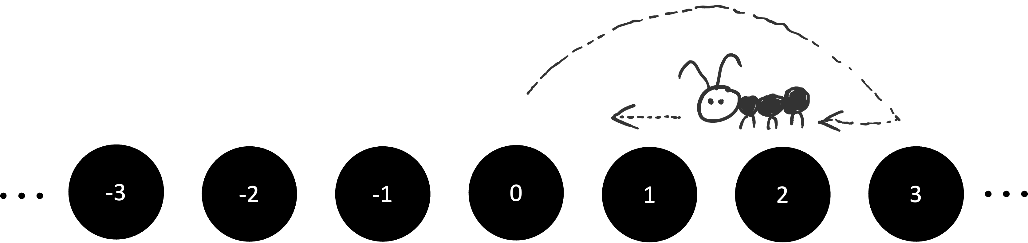
A drunk ant finds his way home…
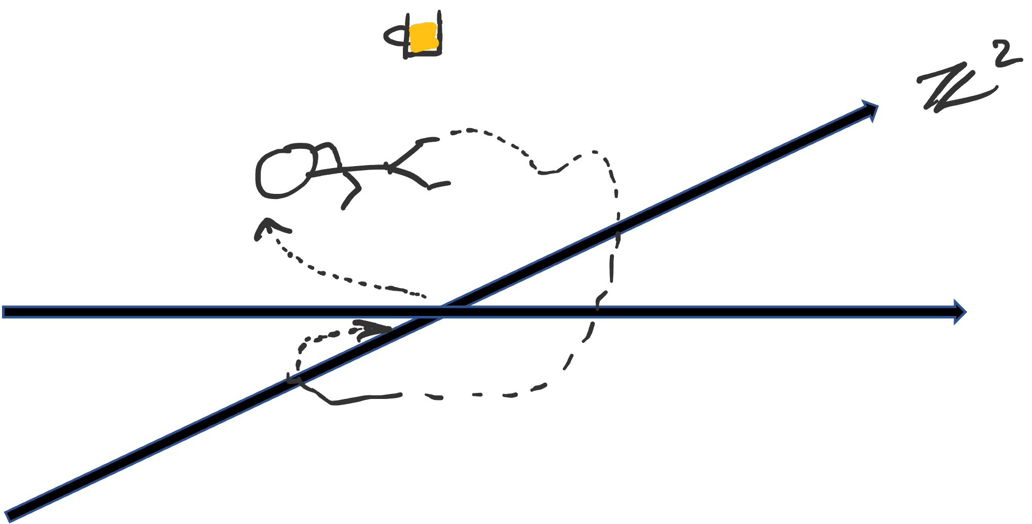
…and so too do does the drunk man (possibly taking a while longer than the ant).
Proof: We note that the simple random walk is symmetric in the sense that any state is equivalent to any other state, so we fix \(x = 0\) and show that \(x = 0\) is recurrent (the proof will then work for any arbitrary state; indeed, it can be shown that any state being recurrent implies all states are recurrent for irreducible Markov chains, but we do not go into this). We prove the results separately for \(d = 1\) and \(d = 2\). Both involve exactly the same idea: do some counting, compute \(\mathbb{E}N_x\) (or, at least, show it must converge) and sprinkle in Stirling’s formula liberally.
For both cases, the random walks are periodic with period 2 in the sense that making a return trip starting and ending at any given state only has positive probability for even steps: that is, \(p_{x,x}^{(2n)} > 0\), where \(p_{x,x}^{(2n)}\) denotes the probability of starting then returning to \(x\) after exactly \(2n\) time-steps. Hence, to find \(\mathbb{E}N_0 = \sum_{n=1}^\infty P(X_{2n} = 0) = \sum_{n=1}^\infty p_{0,0}^{(2n)}\), we simply need to compute \(p_{0,0}^{(2n)}\).
\(d=1\): In order to return to \(0\) after \(2n\) steps, we need to take exactly \(n\) steps forward and \(n\) steps back. There are \(\binom{2n}{n}\) ways of doing this, with \(2^{2n}\) total possible paths (since at each time-step, there are \(2\) possible choices). This gives us
\[p_{0,0}^{(2n)} = \binom{2n}{n} \frac{1}{2^{2n}} \\ = \frac{1}{2^{2n}} \frac{(2n)!}{(n!)^2}.\]Using Stirling’s formula to approximate each factorial, we then have
\[\frac{(2n)!}{(n!)^2} = \frac{\sqrt{4n\pi}\left(\frac{2n}{e}\right)^{2n}}{2n\pi \left(\frac{n}{e}\right)^{2n}} \\ = \frac{2^{2n}}{\sqrt{n \pi}},\]and so
\[p_{0,0}^{(2n)} = \frac{1}{2^{2n}} \frac{2^{2n}}{\sqrt{n \pi}} = \frac{1}{\sqrt{n \pi}}.\]Then
\[\mathbb{E}N_x = \sum_{n=1}^\infty p_{0,0}^{(2n)} = \sum_{n=1}^\infty\frac{1}{\sqrt{n \pi}} = \infty,\]and so the \(d = 1\) simple walk is recurrent, as we wanted to show
\(d = 2\): The proof method is the same. To return to the origin after exactly \(2n\) steps, the walk must balance every “up” step with a “down” step and a “left” step with a “right” step. If there were \(k\) up steps, and hence \(n-k\) left steps, there must be \(k\) down steps and \(n-k\) right steps. The number of ways of this occurring with \(k\) fixed is given by the multinomial
\[\binom{2n}{k,k,n-k,n-k} = \frac{(2n)!}{(k!)^2 ((n-k)!)^2},\]with the total number of paths in \(2n\) steps given by \(4^{2n}\) (since there are \(4\) possible directions to go to in each time-step). Hence, summing over all possible values of \(k\), we get
\[p_{0,0}^{(2n)} = \frac{1}{4^{2n}} \sum_{k=0}^n \frac{(2n)!}{(k!)^2((n-k)!)^2}.\]We can simplify the right-hand side as follows:
\[\frac{1}{4^{2n}} \sum_{k=0}^n \frac{(2n)!}{(k!)^2 ((n-k)!)^2} = \frac{1}{4^{2n}} \sum_{n=1}^\infty \frac{(2n)! (n!)^2}{(n!)^2(k!)^2 ((n-k)!)^2} \\ = \frac{1}{4^{2n}} \binom{2n}{n} \sum_{k=0}^n \frac{(n!)^2}{(k!)^2 ((n-k)!)^2},\]where the summation simplifies to \(\sum_{k=0}^n \binom{n}{k}^2 = \binom{2n}{n}\) (a slick way of seeing this is true is to do the following: pick \(n\) objects from \(2n\) total objects; this can be done in \(\binom{2n}{n}\) ways. Now split the \(2n\) objects into two groups of \(n\) each. We can pick the same \(n\) objects by picking \(i\) from the first group and \(n-i\) from the second group and varying over \(i\). Credits to this post for this proof!). Continuing on, we get
\[p_{0,0}^{(2n)} = \frac{1}{4^{2n}} \binom{2n}{n}^2 = \left(\frac{1}{4^n} \binom{2n}{n}\right)^2,\]and we can use Stirling’s formula to expand the binomial:
\[\frac{1}{4^n} \binom{2n}{n}= \frac{1}{4^n} \left( \frac{(2n)!}{(n!)^2} \right) \approx \frac{1}{4^n} \frac{\sqrt{4\pi n} \left(\frac{2n}{e}\right)^{2n}}{2\pi n \left( \frac{n}{e} \right)^{2n}},\]which simplifies to \(\frac{1}{\sqrt{\pi n}}\). That is to say, we have
\[p_{0,0}^{(2n)} \approx \frac{1}{n \pi} \implies \mathbb{E}[N_0 |X_0 = 0] = \sum_{n=1}^\infty \frac{1}{n\pi} = \infty,\]and we conclude that the two-dimensional simple random walk is also recurrent, as we wanted.
Remark on Theorem 1: If we wanted to be really mysterious, we could say that drunk ants and men will always return home because the infinite sum \(\sum_n \frac{1}{\sqrt{n}}\) and the harmonic series \(\sum_n \frac{1}{n}\) diverges. Of course, there is far more that goes into it than just these divergence results…
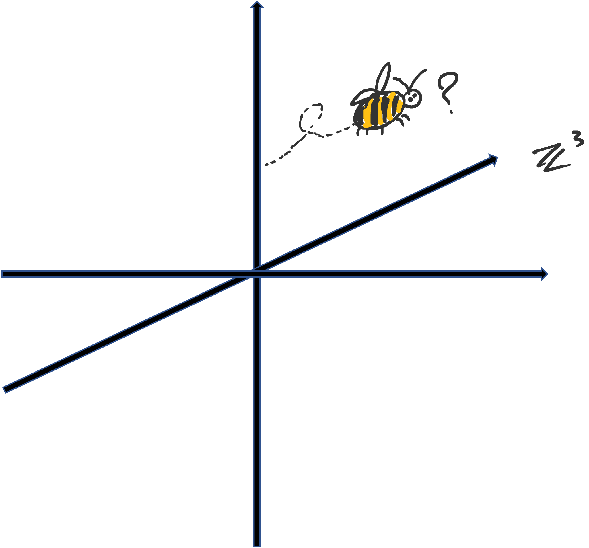
Theorem 2 (Lost drunk bees): The simple random walks on \(\mathbb{Z}^d\) for \(d \geq 3\) are transient. Unfortunately, I will not be providing a proof of this result just yet. You see, proving Theorem 2 is part of an assignment problem set in my stochastic processes course, so after that is completed, I’ll write something up here!
In the meantime, here is a bee: